AstroPaint
A python package for painting the sky
You can install AstroPaint by running the following in the command line:
git clone https://github.com/syasini/AstroPaint.git
cd AstroPaint
pip install [-e] .
the -e argument will install the package in editable mode which is suitable for developement. If you want to modify the code use this option.
Important Note: If you want the sample catalogs to be cloned automatically along with the rest of the repository, make sure you have Git Large File Storage (git lfs) installed.
If you are a conda user, please consider creating a new environment before installation:
conda create -n astropaint python=3.7
conda activate astropaint
Workflow
Converting catalogs to mock maps with AstroPaint is extremely simple. Here is what an example session looks like:
from astropaint import Catalog, Canvas, Painter

catalog = Catalog(data=your_input_data)

canvas = Canvas(catalog, nside)

painter = Painter(template=your_radial_profile)

painter.spray(canvas)
That’s it! Now you can check out your masterpiece using
canvas.show_map()

What is AstroPaint?
AstroPaint is a python package for generating and visualizing sky maps of a wide range of astrophysical signals originating from dark matter halos or the gas that they host. AstroPaint creates a whole-sky mock map of the target signal/observable, at a desired resolution, by combining an input halo catalog and the radial/angular profile of the astrophysical effect. The package also provides a suite of tools that can facilitate analysis routines such as catalog filtering, map manipulation, and cutout stacking. The simulation suite has an Object-Oriented design and runs in parallel, making it both easy to use and readily scalable for production of high resolution maps with large underlying catalogs. Although the package has been primarily developed to simulate signals pertinent to galaxy clusters, its application extends to halos of arbitrary size or even point sources.
Package Structure
While there is no external documentation for the code yet, you can use this chart to understand the package structure and see what methods are available so far.
Examples
Nonsense Template
Here’s an example script that paints a nonsense template on a 10 x 10 [sqr deg]
patch of the Sehgal catalog:
import numpy as np
from astropaint import Catalog, Canvas, Painter

# Load the Sehgal catalog
catalog = Catalog("Sehgal")

# cutout a 10x10 sqr degree patch of the catalog
catalog.cut_lon_lat(lon_range=[0,10], lat_range=[0,10])

# pass the catalog to canvas
canvas = Canvas(catalog, nside=4096, R_times=5)

# define a nonsense template and plot it
def a_nonsense_template(R, R_200c, x, y, z):

    return np.exp(-(R/R_200c/3)**2)*(x+y+z)

# pass the template to the painter
painter = Painter(template=a_nonsense_template)

# plot the template for halos #0, #10, and #100 for R between 0 to 5 Mpc
R = np.linspace(0,5,100)
painter.plot_template(R, catalog, halo_list=[0,10,100])

The painter automatically extracts the parameters R_200c and x,y,z coordinates of the halo from the catalog that the canvas was initialized with. Let’s spray ths canvas now:
# spray the template over the canvas
painter.spray(canvas)

# show the results
canvas.show_map("cartview", lonra=[0,10], latra=[0,10])

Voila!
You can use the n_cpus argument in the spray function to paint in parallel and speed things up! The default value n_cpus=-1 uses all the available cpus.

Stacking
You can easily stack cutouts of the map using the following:
deg_range = [-0.2, 0.2] # deg
halo_list = np.arange(5000) # stack the first 5000 halos

# stack the halos and save the results in canvas.stack
stack = canvas.stack_cutouts(halo_list=halo_list, lon_range=deg_range, lat_range=deg_range)

plt.imshow(canvas.stack)

If this is taking too long, use parallel=True for parallel stacking.
Line-Of-Sight integration of 3D profiles
AstroPaint only allows you to paint 2D (line-of-sight integrated) profiles on your catalog halos, so if you already have the analytical expression of the projected profile you want to paint, we are in business. However, not all 3D profiles can be LOS integrated analytically (e.g. generalized NFW or Einasto, etc), and integrating profiles numerically along every single LOS is generally expensive. In order to alleviate this problem, AstroPaint offers two python decorators @LOS_integrate and @interpolate which make 3D -> 2D projections effortless.
To convert a 3D profile into a 2D LOS integrated profile, all you need to do is add the @LOS_integrate to the definition.
For example, here’s how you can turn a 3D top hat profile
def tophat_3D(r, R_200c):
    """Equals 1 inside R_200c and 0 outside"""

    tophat = np.ones_like(r)
    tophat[r > R_200c]=0

    return tophat
into a 2D projected one:
from astropaint.lib.utilities import LOS_integrate

@LOS_integrate
def tophat_2D(R, R_200c):
    """project tophat_3D along the line of sight"""

    return tophat_3D(R, R_200c)
This function integrates the tophat_3D function along every single line of sight. If you have many halos in a high resolution map, this can take forever. The trick to make this faster would be to integrate along a several LOSs and interpolate the values in between. This is what the @interpolate decorator does. So, a faster version of the tophat_2D function can be constructed as the following:
from astropaint.lib.utilities import interpolate

@interpolate(n_samples=20)
@LOS_integrate
def tophat_2D_interp(R, R_200c):
    """project and interpolate tophat_3D along the line of sight"""

    return tophat_3D(R, R_200c)
This is much faster, but the speed comes at a small price. If your 3D profile is not smooth, the interpolated 2D projection will slightly deviate from the exact integration.
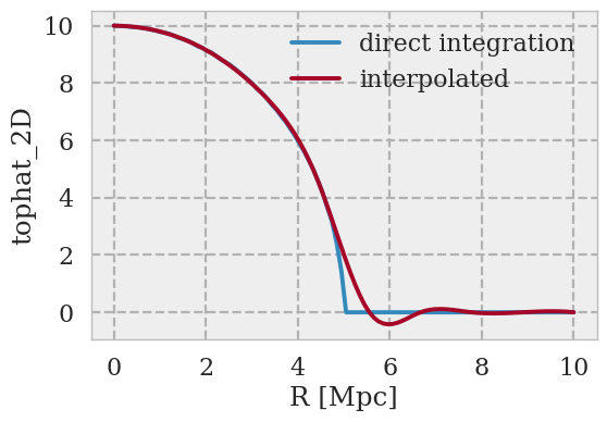
You can minimize this deviation by increasing the n_samples argument of the @interpolate decorator, but that will obviously decrease the painting speed.
Does this plot agree with what you would expect a LOS integrated top hat profile (a.k.a. a solid sphere) to look like?
Painting Optical Depth and kSZ Profiles on the WebSky Catalog
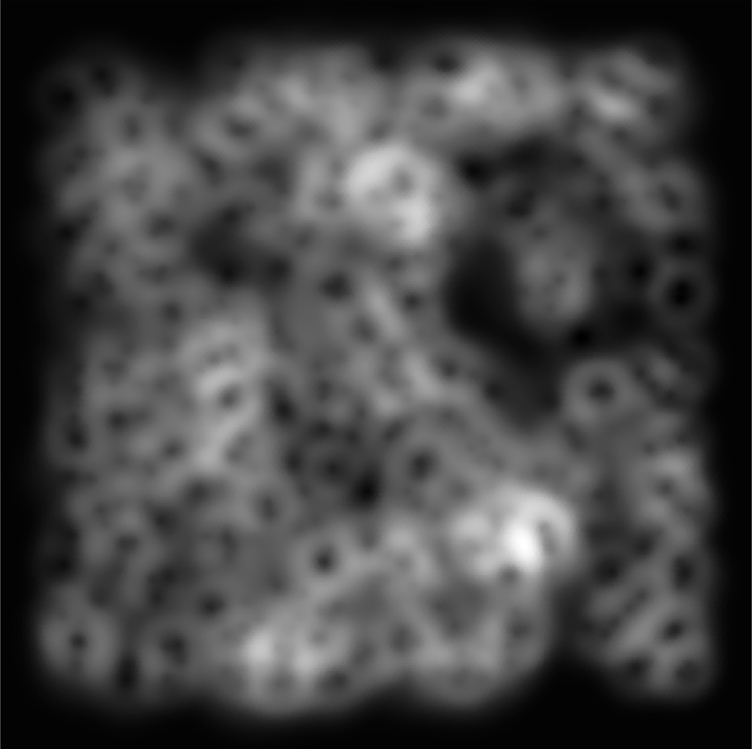
Let’s use the Battaglia16 gas profiles to paint tau (optical depth) and kinetic Sunyaev-Zeldovich (kSZ) on the WebSky catalog halos.
from astropaint.profiles import Battaglia16

 tau_painter = Painter(Battaglia16.tau_2D_interp)
Since the shape of the profile is smooth, we won’t lose accuracy by using the interpolator.

Let’s paint this on a 5x5 sqr deg patch of the WebSky catalog with a mass cut of 8E13 M_sun.
catalog = Catalog("websky_lite_redshift")
catalog.cut_lon_lat(lon_range=[5,10], lat_range=[5,10])
catalog.cut_M_200c(8E13)

canvas = Canvas(catalog, nside=8192, R_times=3)

tau_painter.spray(canvas)

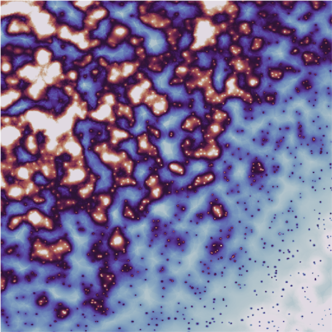
The Battaglia16.kSZ_T function uses this tau and multiplies it by the dimensionless velocity of the halos to get the kSZ signal.
kSZ_painter = Painter(Battaglia16.kSZ_T)
kSZ_painter.spray(canvas)
And here is what it looks like:

Art Gallery
Just because AstroPaint is developed for probing new science and doing serious stuff, it doesn’t mean you can’t have fun with it! Check out our cool web app to get your hands dirty with some paint.
Made with AstroPaint

How to contribute
If you would like to contribute to AstroPaint, take the following steps:
- Fork this repository
- Clone it on your local machine
- Create a new branch (be as explicit as possible with the branch name)
- Add and Commit your changes to the local branch
- Push the branch to your forked repository
- Submit a pull request on this repository
See this repository or Kevin Markham’s step-by-step guide for more detailed instructions.
Developement happens on the develop branch, so make sure you are always in sync with the latest version and submit your pull requests to this branch.
Contents: